Home Enhancing HNSW Efficiency: Cutting Index Build Time by 85%
Home Enhancing HNSW Efficiency: Cutting Index Build Time by 85%
Contents
Optimizing Graph Tradeoffs with Parameter Tuning
Consequences of Slow Index Build Times
Limited Developer Application Experimentation
Slow Update of Dynamic Datasets
Ways to Reduce Index Build Time
Compute-In-Memory (CiM) Associative Processing – Flexible Massive Parallel Processing
The vector database market is growing quickly, with applications like Retrieval Augmented Generation (RAG) for Generative AI (GenAI) and vector similarity search for ecommerce leading the way. Many leading vector database providers use the HNSW (Hierarchical Navigable Small Worlds) algorithm for vector similarity search because it provides fast search with good recall.
This fast search and good recall come at a price, however—it takes a long time to build an HNSW index. Long index build time can lead to issues such as limited scalability, increased operational costs, reduced developer application experimentation, and slow update of dynamic datasets.
Fortunately, there are ways to reduce HNSW index build time. One key approach is to parallelize the nearest neighbor distance calculations needed to build the index. Those calculations represent the longest portion of the index build, so speeding them up is important.
This paper will review the HNSW algorithm, how an HNSW index is built, and why the build time using traditional solutions, like CPU, takes a long time. It will also present a solution that leverages a high degree of parallelism to reduce index build time by roughly 85% compared to CPU.
A report from MarketsandMarkets™ 1 forecasts the vector database market to grow from $1.5 billion in 2023 to $4.3 billion by 2028, representing a CAGR of 23.3%.
RAG is one of the main drivers of this growth. RAG retrieves relevant documents from a large corpus and uses those documents in GenAI applications to generate a response. By incorporating this external information, it allows for more accurate and reliable responses and reduces hallucinations, where inaccurate responses are given that are not based on factual information.
RAG leverages vector databases to efficiently store and retrieve those relevant documents, which are in the form of vector embeddings. The need for effective and efficient retrieval of vector embeddings has made vector databases integral to RAG.
Additionally, RAG is contributing to the trend of billion-scale vector databases. That is because larger datasets provide a wider range of information to retrieve relevant information from. Cohere,2 a leading provider of LLMs, states that some of their customers scale to tens of billions of vector embeddings.
Another application that is driving the need for billion-scale vector databases is ecommerce. For example, eBay3 stated that their “marketplace has more than 1.9 billion listings from millions of different sellers.” Those listings are in the form of vector embeddings that the vector database stores and retrieves as part of the recommendation process.
Within the vector database market, HNSW is one of the most popular Approximate Nearest Neighbor (ANN) algorithms used to search and retrieve vector embeddings. It has been adopted by many vector database providers like Vespa4 and Weaviate5 and by companies like AWS6 and eBay.7
HNSW is a graph-based algorithm that efficiently searches for the approximate nearest neighbors of a query. The graph is hierarchical, meaning it has multiple layers of nodes (vector embeddings), where each layer contains a subset of the previous layer. The nodes are connected by edges, which represent the distance between them. Distance is measured by a metric, such as cosine similarity.
The higher layers have fewer nodes and longer edges between the nodes, which allows for bridging distant regions of the graph. The bottom layer includes all the vectors and has short-range edges (connecting to nearby nodes).
Figure 1 provides a simple example of an HNSW graph structure.
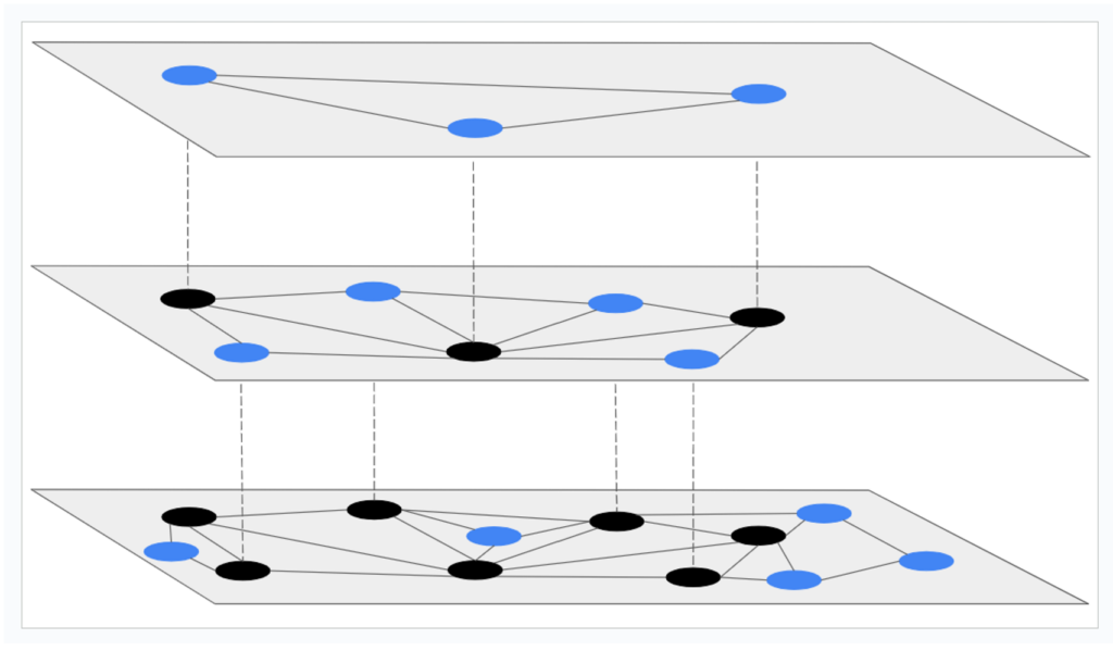
Figure 1: Example HNSW graph showing the hierarchical layers structure. The top layer has the fewest nodes and longer connections, while the bottom layer contains all the nodes and has short-range edges.
This multi-layered graph structure with fewer, long-range connections on the top layers and denser, short-range connections on the bottom layers allows for a coarse-to-fine search approach. This provides faster pruning of irrelevant portions of the graph during nearest neighbor search, resulting in reduced search time.
The fewer nodes and longer edges in the top layers allow fast exploration of the vector space, while the denser nodes and shorter edges in the lower layers allow for more refined searches.
The HNSW search algorithm starts by taking big jumps across the top layers and progressively moving down the hierarchy of layers to refine the search. This minimizes the number of distance calculations needed, speeding up similarity searches.
This approach is analogous to the steps one might take in searching for a specific house. You start at the city level, then move to a specific neighborhood, a particular street, and finally, you find the house you are looking for.
The long-range connections in the top layers act like shortcuts, and they ensure the “small world” property of the graph. This means most nodes can be reached in a few hops. This concept is shown in Figure 2—a long-range connection is used to help find the nearest neighbor for the query in two hops from the entry point.
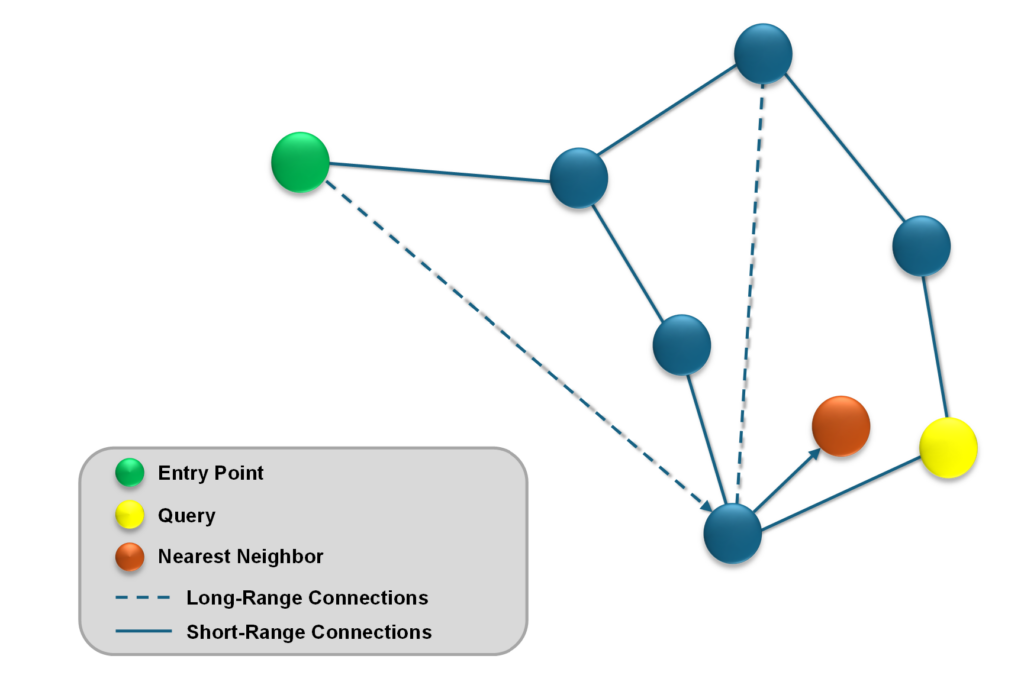
Figure 2: “Small world” concept demonstrated where a long-range connection allows for an efficient 2-hop graph traversal from the Entry Point to the Query’s nearest neighbor.
Parameters M and ef_construction, which are both related to the number of links a node has in the HNSW graph, help optimize the trade-off between index build time, memory usage, and accuracy.
During index build or update, new nodes are inserted into the graph based on their distance from existing nodes. At each layer, a dynamic list of the nearest neighbors seen so far is kept. The parameter ef_construction determines the size of this list.
The index build algorithm iterates over the nodes in the list and performs nearest neighbor distance calculations to see if the nodes’ neighbors are closer to the query than they are, and if so, considers adding the nodes’ neighbors to the dynamic list.
A larger ef_construction means that more candidates are tracked and evaluated, increasing the chance of finding the true nearest neighbors for each node in the graph. This improves accuracy, but increases the index build time since more distance calculations are needed.
Similarly, increasing M, which is the number of bi-directional links created for each node in the graph, improves the accuracy of the graph but also increases the build time since more distance calculations and updates are needed.
By tuning the values of M and ef_construction, developers can experiment with different indexes to optimize the specific requirements of their application. For example, they can tune the values to prioritize index build time over accuracy or vice versa.
As seen in the previous sections, building an HNSW index is a compute-intensive process that requires a lot of distance calculations to find the nearest neighbors for each vector in a hierarchy of graph layers. While this results in a graph with low search latency and good recall, it also comes with the tradeoff of a graph that is slow to build and update.
For example, as seen in Figure 3, eBay found that building an HNSW graph for an index size of 160M vectors can take about 3 hours to 6 hours based on the different parameters chosen.
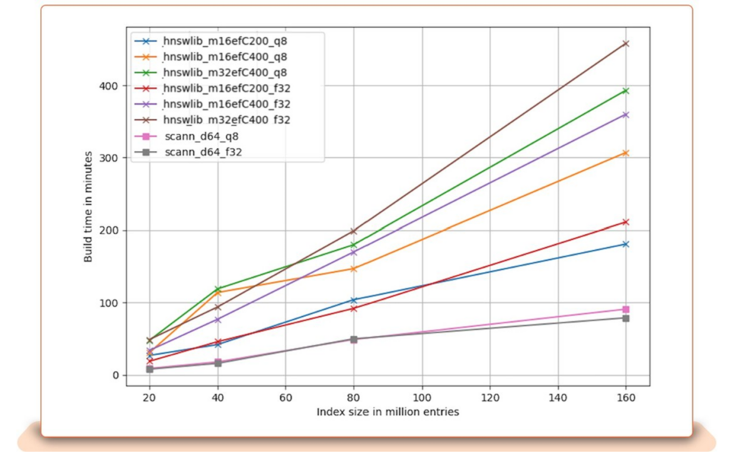
Figure 3: Index build time vs. index size. Different quantization, M, and ef_construction values are used.7
The figure also shows that build time increases rapidly as the number of vectors in the index grows. This can be problematic for a company such as eBay that, as mentioned earlier, has billions of live listings.
Slow index build times can lead to many challenges, such as: scalability issues, increased operational costs, limited developer application experimentation, and slow update of dynamic datasets.
Slow index builds can limit a company’s ability to scale. Two examples of this can be seen in ecommerce and RAG:
With vector search applications scaling to billions of items, slow index build time can lead to increased operational costs, which lowers profit margins. For example:
As mentioned earlier, developers experiment with different parameters, such as M and ef_construction, to test different indexes and tune the performance of their application.
In a post, eBay commented on the importance of being able to experiment quickly — “Our ML engineers develop many ML embedding models as they iterate on their hypotheses for improved features. Any time there is a change in the ML model, even when it’s a small feature or a new version, the vector space of embeddings changes and therefore a new vector search index needs to be created…. Rapid ML model iteration is ultimately what brings value to the end user by an improved recommendations experience.”3
Longer index build time impacts this ability to experiment in a few ways:
Applications like ecommerce and RAG have dynamic datasets where new products or information is frequently added to the database. Long index build time delays updates to this dynamic data, affecting the system’s relevancy and accuracy of search results.
Two effective ways to reduce index build time are parallel processing and compressing the vectors through quantization.
A few ways to use parallel processing to reduce index build time are to:
Unfortunately, CPUs, which most HNSW index build solutions use, have limited parallel processing capabilities. While some high-end multi-core CPUs have 64 cores that can perform parallel processing, this is still a small number of cores. This limits the number of parallel operations they can perform, so they can only process a minimal amount of vectors at a time.
What is needed is a solution with massive parallel processing capability.
Compressing the vectors in the index through quantization speeds up the build time by:
What is needed is a flexible solution that can work with quantized vectors of varied bit lengths. This allows for experimenting with different compression algorithms to see which bit length is optimal for achieving a particular set of goals, such as build time or accuracy.
GSI Technology’s compute-in-memory Associative Processing Unit (APU) is a technology that allows for massive parallel processing and flexible quantization. It is based on bit-level processing, and computation is done in place, directly in memory, which avoids the traditional bottleneck between processors and memory.
Building an index with the APU involves the following steps:
The APU has millions of bit processors that perform computation at the bit level. This allows for massive parallel processing on any sized data element.
The APU’s bit-level processing allows each data bit to be processed independently. For example, for a 16-bit data item, each of the 16 bits can be processed individually.
The APU architecture stores the corresponding bits of multiple data elements together. For the 16-bit example mentioned above, this means the first bits of a set of 16-bit numbers are stored together, all the second bits together, etc. This can be seen in Figure 4, where Bit Slice 0 holds all the 0 bits for each 16-bit data item, Bit Slice 1 holds all the 1 bits, etc.
All the data elements for each bit slice are accessed in parallel, which coupled with the millions of bit processors, allows for massive parallel processing.
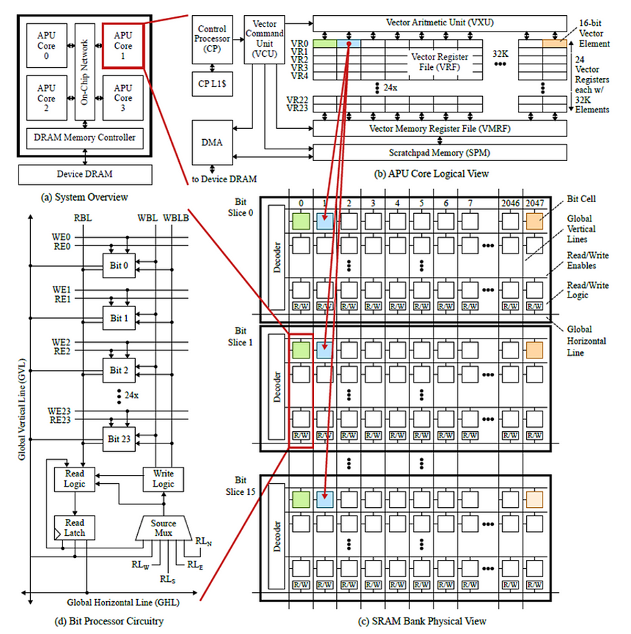
Figure 4: The APU’s bit-parallel architecture stores the corresponding bits of multiple data elements together. For example, Bit Slice 0 holds the 0 bits for each data item in a set of items.8
The APU takes advantage of this bit-level processing and massive parallel processing to speed up the index build process detailed earlier:
Figure 5, from Nvidia, shows that an Intel Xeon Platinum 8480CL CPU takes 5,636 seconds (about 1 and a half hours) to build an HNSW index for 100M vectors.
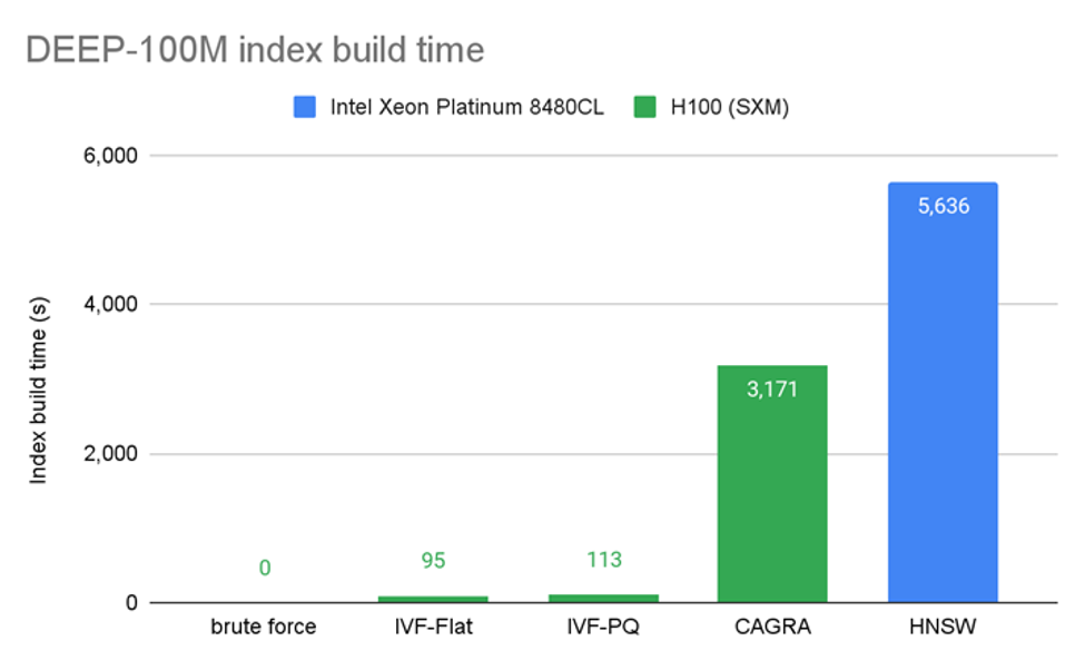
Figure 5: CPU HNSW index build time for 100M vectors9
Figure 6 presents the HNSW index build times using an APU system for datasets ranging from 100 million vectors to 1 billion vectors. It shows an APU system can build a 100 million vector index in 864 seconds (about 15 minutes). This represents nearly an 85% reduction in build time compared to the 5,636 seconds (about 1 and a half hours) for an Intel Xeon Platinum 8480CL CPU.
Figure 6 also shows that an APU system can build a 1 billion vector HNSW index in 7800 seconds (about 2 hours), which is a significant improvement compared to Figure 3 from eBay if the eBay build times were extrapolated to 1 billion vectors.
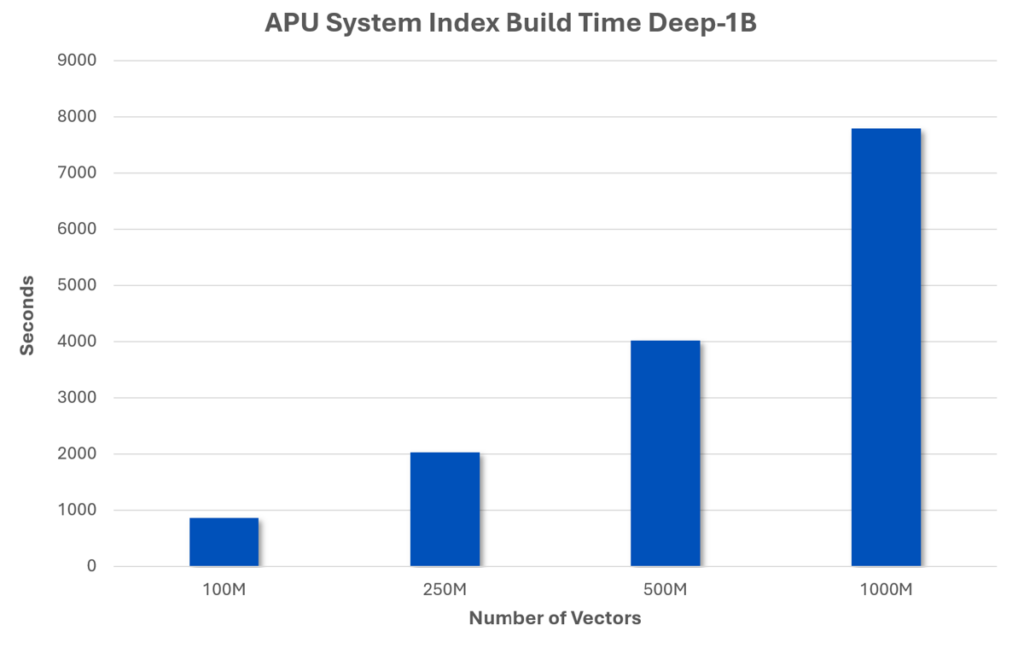
Figure 6: HNSW index build time for 100 million–1 billion vectors.
This fast index build time has many benefits:
In RAG applications, it allows the latest information to be accessed sooner, leading to more relevant and accurate responses.
HNSW is a leading algorithm used for vector similarity search in applications like GenAI and ecommerce. It provides high recall and fast search, but with the tradeoff of long index build time.
Long index build time limits scalability, increases costs, leads to less experimentation, and delays updates to dynamic data. This lowers a company’s growth potential, reduces profits, leads to less innovation, and erodes customer confidence if incorrect or irrelevant responses are generated.
One of the main ways to reduce index build time is through parallelization. Unfortunately, most current solutions use CPUs, which have limited parallel processing capabilities.
GSI’s APU addresses this issue by providing massive parallel processing. The APU’s millions of bit processors allow for massive parallel computation of the many nearest neighbor distance calculations needed to build an index. The nearest neighbor distance calculations are the longest step in building an index, so performing them in parallel significantly reduces index build time.
The result—roughly an 85% reduction in index build time compared to traditional CPU-based solutions.
To find out more about how GSI Technology’s on-prem and cloud-based offerings can significantly reduce your HNSW index build times, contact us at [email protected].