- ABOUT GSI
- AI
- HPC
- INDUSTRIES
- AEROSPACE & DEFENSE
- MEMORY
- RESOURCES
- INDEPTH
-
-
AI’s Energy Dilemma

-
-
- INTEGRATORS
-
- TOOLS
-
- INDEPTH


Home An Overview of Model Compression Techniques for Deep Learning in Space
Authors: Hannah Peterson and George Williams

Every day we depend on extraterrestrial devices to send us information about the state of the Earth and surrounding space—currently, there are about 3,000 satellites orbiting the Earth and this number is growing rapidly. Processing and transmitting the wealth of data these devices produce is not a trivial task, given that resources in space such as on-board memory and downlink bandwidth face tight constraints. In the case of satellite images, the data at hand can be extremely large, sometimes as large as 8,000×8,000 pixels. For most practical applications, only part of the great amount of detail encoded in these images is of interest—such as the footprints of buildings, for example—but the current standard approach is to transmit the entire images back to Earth for processing. It seems a more efficient solution would be to process the data on board the spacecraft, arriving at a compressed representation that occupies fewer resources—something that could be achieved using a machine learning model.
Unfortunately, running machine learning models tends to be a resource-intensive process even here on Earth. State-of-the-art networks typically consist of many millions of parameters and limited uplink bandwidth makes uploading such large networks to satellites impractical/infeasible. And even if they were pre-loaded prior to launch, they require significant memory bandwidth to fetch weights and compute dot products at runtime. Energy consumption of these networks is dominated by memory accesses, and they typically rely on hardware accelerators for timely inference. Spacecraft, however, face very strict weight and power requirements, which means that a satellite can’t be loaded with an unlimited number of GPUs for the purpose of running a model.
In this way, the topic of model compression is particularly relevant to space-based applications, as there is an evident need to reduce the size and complexity of neural networks for deployment in highly constrained extraterrestrial environments. Luckily, many effective techniques for model compression exist thanks to a rapidly growing body of research on the topic. In this blog, I’ll be going over a few common approaches.
The goal of model compression is to achieve a model that is simplified from the original without significantly diminished accuracy. A simplified model is one that is reduced in size and/or latency from the original. Specifically, a size reduction means that the compressed model has fewer and/or smaller parameters and, thus, uses less RAM when run, which is desirable because it frees up memory for other parts of the application to use. A latency reduction is a decrease in the time it takes for the model to make a prediction, or inference, based on an input to the trained model, typically translating to lower energy consumption at runtime. Model size and latency often go hand-in-hand because larger models require more memory accesses to be run. As we can see, both types of reduction are desirable for deploying models in space, where computing resources face both strict size and power constraints.
The following are some popular, heavily researched methods for achieving compressed models:
Let’s take a look at each technique individually. In practice, a complete model compression pipeline might integrate several of these approaches, as each comes with its own benefits and drawbacks.
Pruning involves removing connections between neurons or entire neurons, channels, or filters from a trained network, which is done by zeroing out values in its weights matrix or removing groups of weights entirely; for example, to prune a single connection from a network, one weight is set to zero in a weights matrix, and to prune a neuron, all values of a column in a matrix are set to zero. The motivation behind pruning is that networks tend to be over-parametrized, with multiple features encoding nearly the same information. Pruning can be divided into two types based on the type of network component being removed: unstructured pruning involves removing individual weights or neurons, while structured pruning involves removing entire channels or filters. We’ll look at these two types individually, as they differ in their implementations and outcomes.

By replacing connections or neurons with zeros in a weights matrix, unstructured pruning increases the sparsity of the network, i.e. its proportion of zero to non-zero weights. There exist various hardware and software, such as TensorFlow Lite and Caffe, that are specialized to efficiently load and perform operations on sparse matrices and, thus, that can facilitate significant latency reductions in pruned models as compared to their original dense representations. For example, Caffe can be used to apply a mask to pruned parameters that causes them to be skipped over during network operation, reducing the amount of FLOPs and, thus, the power and time, required to make an inference. Depending on the degree of sparsity and the method of storage used, pruned networks can also take up much less memory than their dense counterparts.
But what is the criteria for deciding which weights should be removed? One common method known as magnitude-based pruning compares the weights’ magnitudes to a threshold value. A highly cited 2015 paper by Han et al. prompted widespread adoption of this approach. In their implementation, pruning is applied layer-by-layer. First, a predetermined “quality parameter” is multiplied by the standard deviation of a layer’s weights to calculate the threshold value and weights with magnitudes below the threshold are zeroed. After all layers are pruned, the model is retrained so that the remaining weights can adjust to compensate for those that were removed, and the process is repeated for several iterations. The researchers used this method to prune four different model architectures, two pre-trained on the MNIST dataset and two on the ImageNet dataset. We can see the effects of their unstructured pruning approach visualized in the following image, which shows the sparsity pattern of the first fully-connected layer for one of the MNIST networks, where the blue dots represent non-zero parameters:

The MNIST dataset consists of 28×28 pixel images of handwritten digits from 0–9 like the one above and models are trained to classify these digits. To be inputted into a neural network, the image is flattened by concatenating the rows of pixels end-to-end from top to bottom, resulting in a vector of 784 values. The first layer of the network is fully-connected with 300 neurons. As we can see, the digits tend to be oriented in the center of the image, thus pixels around the edges are less consequential to the classification task and connections to them get pruned more heavily. For the entire network, pruning caused both the number of non-zero weights and FLOPs required to decrease by a factor of 12 with no drop in predictive performance. Similarly, for the AlexNet and VGG-16 models trained on ImageNet, the numbers of parameters were reduced from 61 million to 6.7 million and from 138 million to 10.3 million, respectively, with no decrease in classification accuracy.
Han et. al showed that when implemented correctly, unstructured pruning can yield some truly impressive degrees of compression, as they note “the storage requirements of AlexNet and VGGNet are are small enough that all weights can be stored on chip, instead of off-chip DRAM which takes orders of magnitude more energy to access.” However, they also acknowledge the “limitation of general purpose hardware on sparse computation” and, thus, use specialized software to work around this problem. Indeed, unstructured pruning’s reliance on specially designed software or hardware to handle network sparsity to speed up computations is a significant limitation, one that is not faced by taking a structured approach.

Unlike unstructured pruning, structured pruning does not result in weight matrices with problematic sparse connectivity patterns because it involves removing entire blocks of weights within given weight matrices. This means the pruned model can be run using the same hardware and software as the original. While we are now looking at groups of weights to remove at the channel or filter level, magnitude-based pruning can still be applied by ranking them according to their L1 norms, for example. But there are also more intelligent, “data-driven” approaches that have been proposed which can achieve better results.
Huang et al., for example, were the first to integrate into the pruning process a means of controlling the tradeoff between network performance and size in their 2018 paper. Their algorithm outputs a set of filter “pruning agents”—each a neural network corresponding to a convolutional layer of the network—and an alternative, pruned version of the original model, which is initialized to be the same as the original. The pruning agents work to maximize an objective that is parametrized by a “drop bound” value, which is defined as the maximum allowed drop in performance between the original and the pruned model, forcing the agents to keep performance above a specified level. For each convolutional layer, a pruning agent is trained by evaluating the effects of pruning combinations of different filters within that layer. To do so, it removes certain filters from the alternative model and compares this model’s performance on an evaluation set to that of the original, learning which modifications will increase the network’s efficiency while still adhering to accuracy constraints. Once the agent for one layer is trained and filters for that layer have been optimally removed, the entire pruned model is retrained to adjust for the changes and the process repeats for the next convolutional layer.
The following plot shows the degree of pruning achieved with this approach with drop bound b = 2 on the layers of a VGG-16 model trained on the CIFAR 10 dataset. The greater degree of pruning of higher layers indicates they tend to contain more unnecessary filters than initial ones.

We can also see the quantitative compression results of pruning this model using different drop bound values. The accuracy values in parentheses correspond to models pruned to the same ratio but with a magnitude-based approach instead, and we see that the “data-driven” implementation has superior performance.

Similarly impressive results have been achieved through a variety of structured pruning methods, establishing it as a popular model compression technique. But pruning in general still has a few potential drawbacks. For example, it’s generally unclear how well given methods generalize across different architectures, and the pruning process tends to involve a lot of fine-tuning that can act as a barrier both to implementation and generalization. Further, in many cases it may be more effective to simply use a more efficient architecture than to prune a suboptimal one. If you’re interested in taking a closer look at the diverse range of approaches currently being taken to prune models, I suggest checking out this blog or the paper “What is the State of Neural Network Pruning?”, both written in 2019.

While pruning compresses models by reducing the number of weights, quantization consists of decreasing the size of the weights that are there. Quantization in general is the process of mapping values from a large set to values in a smaller set, meaning that the output consists of a smaller range of possible values than the input, ideally without losing too much information in the process. We can think about this in the context of image compression, as with the images of Einstein above. In the leftmost representation, each pixel value is represented by 8 bits and thus can take on 256 varying shades of gray. The number of possible shades is halved in each successive image. Notice, however, that we really aren’t able to detect much difference between the first four images or so, and this represents the goal of model quantization: to reduce the precision of network components to the extent that it is more lightweight but without a “noticeable” difference in efficacy. Intuitively, it makes sense that neural networks should be able to deal with some information loss, as they are trained to cope well with high levels of noise in their inputs, and lower precision calculations can essentially be seen as another source of noise.
So, how might a mapping between different precisions (i.e. a quantization scheme) work? In a neural network, the weights or activation outputs of a particular layer tend to be normally distributed within a certain range, so ideally a quantization schema takes advantage of this fact and adapts to fit each layer’s individual distribution. For example, models weights are typically stored as 32-bit floating point numbers and a common approach is to reduce these to 8-bit fixed points (though some techniques have even gone as far as to represent them with single bits!), for which there are 2⁸ = 256 possible values: in the simplest case, we can take the min and max weights of a layer, divide the range between the two into 255 evenly-spaced intervals, and bin the weights according to the interval edge they are closest to:

We can see how quantizing the weights in this way would reduce their memory footprint by 4x. And there are many other, more complex techniques that achieve lower information loss, such as an implementation by Han et. al that involves k-means clustering. Specifically, their compression pipeline combines weight pruning, quantization, and Huffman coding, and we can see in the following graph how pruning and quantization of AlexNet trained on ImageNet work together to achieve a model that is 3.7% of its original size with no loss in accuracy:

In addition to weights, neural networks also consist of operators such as matrix multiplication, convolution, activation functions and pooling that must also be quantized to deal with lower precision weights. While the general idea is the same, quantizing operators is a bit trickier than quantizing pre-trained weights because they have to deal with potential bit overflows and unseen inputs, which can make determining a schema difficult. Luckily, many deep learning softwares, such as TensorFlow, PyTorch, and MXNet, have functionality for quantizing commonly-used operators (if you’re interested, this blog provides high level explanation of TensorFlow’s process), which can yield networks with significantly diminished latency given the increased efficiency of lower precision operations.
In practice, quantization can be difficult to actually implement because it requires having a decent understanding of hardware and bit-wise computations. It turns out that deciding upon the degree of precision to compress a model to is not as simple as picking a random number of bits: you have to make sure the hardware you’re using is even capable of handling numbers of that size, let alone of doing so efficiently. In reviewing the literature, I found that the savings offered by many state-of-the-art quantization implementations are tied to the features of the hardware being used, although here exist other means of compression that generalize well across many kinds of hardware, such as low-rank factorization.

We’re aware that deep neural networks tend to be over-parametrized, with a lot of similarity—or redundancy—occurring between different layers and/or channels. For example, image a above shows filters of a convolutional layer learned for an image segmentation task, many of which look nearly the same. The goal of low-rank approximation is to approximate the numerous, redundant filters of a layer using a linear combination of fewer filters, such as those represented in image b. Compressing layers in this way reduces the network’s memory footprint as well as the computational complexity of convolutional operations and can yield significant speedups.
Specifically, the filters in b are of lower rank than those in a. The rank of a matrix is defined as the dimension of the vector space spanned by its columns, which is equal to its number of linearly-independent columns. To illustrate, say we have the following matrix:
[[1, 0, -1],
[-2, -3, 1],
[3, 3, 0]]
If we look at just the first two columns, we see that they are linearly independent because neither can be computed from the other using linear operations, so the matrix has to have a rank of at least 2. But if we look at all three columns, we see that if we subtract the first from the second, we get the third, thus all three are not linearly independent and the matrix only has a rank of 2.
Intuitively, we get the sense that if an element of a matrix can be computed using others that are present, there is some redundancy of information occurring in the matrix. While individual filters and channels in a network tend to be full rank, indicating no redundancy within themselves, there is typically significant redundancy between different filters or channels. And since low-rank matrices encode redundant information, it makes sense that we can use them to approximate these redundant layers of a network, which is exactly what low-rank approximation does. To understand the intuition behind how this might be achieved, let’s take a look at a relatively simple approach from Jaderberg et al. that takes advantage of cross-filter redundancy.
The following represents a convolution operation with N 2D filters, W, on a single channel feature map, Z, to output an N-channel feature map.

The goal is to reduce the computational complexity of these operations by approximating the N full rank filters with a linear combination of M lower rank filters where M<N, based on the assumption that there is redundancy between the N filters. Specifically, Jadenberg et al. impose that the new filters be of rank 1. If a matrix has rank 1, it means that if we select one of its columns, all the other columns will be some multiple of that column. Thus, rank 1 matrices can be factorized or decomposed to be products of a column vector and a row vector—a property called separability—for example:
[[1, 4, 5],          [[1],   [[1, 4, 5]]
[2, 8, 10],     =     [2], *
[3, 12, 15]]          [3]]
By imposing separability of the M basis filters and adding a layer to approximate the N output channels of the original convolution operation from the compressed basis, we arrive at a transformed operation that looks like this:

While it may look more complex, it is actually a more computationally efficient operation if M is made to be sufficiently small. The separable bases for these modified layers are optimized asynchronously by minimizing the reconstruction error between the output of the original layer and the output of the approximation layer. Jaderberg et al. use a similar approach to exploit redundancy between channels, with which they achieve 4.5× speedup of a shallow network trained for a text classification task with only a 1% drop in classification accuracy.
If you take a look at the literature on low-rank approximation, it’s likely you’ll come across the terms SVD (“Singular Value Decomposition”), Tucker decomposition and CP (“Canonical Polyadic”) decomposition, so it bears briefly explaining the designation between these. SVD stands for “Singular Value Decomposition” and is a matrix factorization. In the context of approximating a matrix M with another matrix M’ of a lower rank r as we’ve discussed, the optimal M’ is equal to the SVD of M constrained by r. Tucker and CP decomposition are ways of generalizing SVD to tensors. As you likely know, a tensor is a multi-dimensional array. Tucker decomposition decomposes a tensor into a set of matrices and one small core tensor. CP is actually a special case of Tucker decomposition that decomposes a tensor into a sum of rank-1 tensors, though they are often referred to in the literature as two separate approaches. We can see how they both work in 3D space below:

Both have their benefits and drawbacks, which you can read more about here, and are popular approaches to low-rank approximation of deep neural networks. Kim et al., for example, achieve substantial compression using Tucker decomposition. They take a data-driven approach to determining the ranks that the compressed layers should have and then perform Tucker decomposition according to these ranks. They apply this compression to various models for image classification tasks and run them on both a Titan X and Samsung Galaxy S6 smartphone, which, notably, has a GPU with 35× lower computing ability and 13× smaller memory bandwidth than Titan X. The following table shows the compressed models’ drops in performance and reductions in size and FLOPs from the original, as well as their time and energy consumption to process a single image.

With these results, Kim et al. demonstrate that low-rank approximation is an effective means of compression to achieve significant size and latency reductions in deep neural networks for their potential deployment on mobile devices. And as I mentioned before, a large upside to low-rank approximation as a compression technique is that, since it simplifies model structure just by reducing parameter count, it does not require specialized hardware to implement.
If we think about it, the need to compress neural networks arises from the fact that training and inference are two fundamentally different tasks. During training, for example, a model does not have to operate in real time and does not necessarily face restrictions on computational resources, as its primary goal is simply to extract as much structure from the given data as possible, but latency and resource consumption do become of concern if it is to be deployed for inference. As a result, trained models are often larger and slower than what would be ideal for inference and, hence, we have to develop ways compress them. To address this problem, Cornell researchers proposed in 2006 the idea of transferring the knowledge from a large trained model (or ensemble of models) to a smaller model for deployment by training it to mimic the larger model’s output, a process that Hinton et al. generalized in 2014 and gave the name distillation. In short, knowledge distillation is motivated by the idea that training and inference are different tasks such that a different model should be used for each.

In Hinton et al.’s implementation, the small “student” network learns to mimic the large “teacher” network by minimizing a loss function in which the target is based on the distribution of class probabilities outputted by the teacher’s softmax function. To understand this, let’s review how the softmax function works: it takes in a a logit for a particular class, z_i, and converts it to a probability by dividing it by the sum of logits of all j classes:

Here, the term T is the temperature, of which higher values correspond to “softer” outputs. T is usually set to 1, which results in “hard” outputs in which the correct class label is assigned a probability close to 1, indicating near certainty in this prediction, while the others are assigned probabilities close to 0. Hinton et al. suggest, however, that the distribution of the incorrect class labels holds valuable information about the data that can to be learned from, as they describe in the context of a handwritten digit classification task:
“One version of a 2 may be given a probability of 10^-6 of being a 3 and 10^−9 of being a 7 whereas for another version it may be the other way around. This is valuable information that defines a rich similarity structure over the data (i. e. it says which 2’s look like 3’s and which look like 7’s)…”
To capitalize upon this information, Hinton et al. raise the temperature T in the teacher network’s softmax function to soften the distribution of probabilities over the class labels in a process they call distillation, as demonstrated in the following:

The student network is then trained to minimize the sum of two different cross entropy functions: one involving the original hard targets obtained using a softmax with T=1 and one involving the softened targets. Hinton et al. demonstrate the effectiveness of this technique by training a teacher network with two hidden layers of 12,000 units and a student with two hidden layers of only 800 units. On a test set, the teacher achieves 67 test errors and the student achieves 74, as compared to the 146 test errors made by a network of the same size as the student but that was trained without distillation.
After this initial breakthrough by Hinton et al. of training the student to imitate the softmax outputs of a teacher, researchers Romero et al. found that the student can also use information from the teacher’s intermediate hidden layers to improve its final performance. Specifically, they propose what they call “FitNets,” which are student networks that are thinner but deeper than their teachers, with their increased depth allowing them to generalize well while their small widths still make them compact. Romero et al. introduce one “guided layer” in the middle of the student network that is tasked with learning from one “hint” layer in the middle of the teacher network. The table below demonstrates the speedup, reduced parameter count, and generally increased accuracy the FitNets of varying sizes achieve as compared to their teacher architecture on the CIFAR-10 image classification dataset. Further, their performance was on-par with state-of-the-art methods, of which the highest accuracy at the time was 91.78%:

Impressive results like these have spurred research on a wide range of different methods for transferring knowledge from teacher to student networks. Indeed, the field of research on knowledge distillation has become so broad and specialized in some areas that it is difficult to evaluate the overall efficacy of general approaches against one another. A drawback of knowledge distillation as a compression technique, therefore, is that there are many decisions that must be made up-front by the user to implement it; for example, unlike the other compression techniques we’ve discussed, the compressed network doesn’t even need to have a similar structure to the original. But this also means that knowledge distillation is very flexible and can be adapted to a wide range of tasks. If you’re interested in learning more about different knowledge distillation techniques, this 2020 paper performs a comprehensive review of state-of-the-art approaches for vision-based tasks.
The reality is that multiple of the compression techniques we’ve discussed so far could be applied in a given scenario, and when you take into account combinations of them, the number of possible architectures to explore expands dramatically. The hard part is, of course, choosing the optimal one. This is where Neural Architecture Search (NAS) comes in. NAS in the most general sense is a search over a set of decisions that define the different components of a neural network—it is a systematic, automized way of learning optimal model architectures. The idea is to remove human bias from the process to arrive at novel architectures that perform better than human-designed ones.
Obviously, for any given task there are infinite possible model architectures to explore and, with this, many different approaches to searching through them. A 2019 survey categorizes different NAS techniques according to the following three dimensions:

Search space: The possible architectures that can be discovered in the search. We’re aware that networks can consist of a whole host of operations such as convolutions, pooling, concatenation and activation functions, and defining a search space involves imposing constraints on how and which of these components can be combined to generate the networks that are searched through. For example, defining a search space might involve restricting the number of possible convolutional layers the network can have or requiring it to repeat a general pattern of operations several times. Inevitably, imposing such restrictions introduces some human bias into the search process. And even with these restrictions, the search space will still be very large, as is the point of NAS — to discover and evaluate architectures outside of the realm of what we might normally construct.

Search strategy: The strategy followed to guide the exploration of the search space, i.e. what determines the next architectures to explore in the search. While this could be random, it’s unlikely given the huge scope of a given search space that an optimal architecture will be happened upon by random chance, so the search strategy typically takes into account the performance of previously explored architectures. For example, so-called “evolutionary” algorithms are based on maintaining an evolving population of candidate architectures throughout the training process. There are also reinforcement-learning-based strategies where an agent is trained to estimate the performance of architectures on unseen data.
As you can imagine, NAS is a very broad field of research, so here we will just focus on its use for compressing pre-trained models, specifically. In 2018, for example, He et al. introduced AutoML for Model Compression (AMC), a technique that uses a reinforcement learning search strategy to compress pre-trained networks layer-by-layer. Specifically, AMC’s search space is parametrized by a user-defined, hardware-based constraint such as maximum latency, model size, or number of FLOPS. The agent proceeds through the network one layer at a time, outputting a compression ratio that is based on the composition of the layer and that also adheres to the hardware constraint. After all layers are pruned according to their ratios via a structured or unstructured approach, the validation accuracy of the compressed model is computed without fine-tuning and used as the agent’s reward. Forgoing fine-tuning after compressing the model is a tactic He et al. take in their performance estimation strategy that allows for faster policy exploration.
AMC’s learning-based pruning was tested against handcrafted, rule-based approaches on various models and was found to exhibit all-around superior performance. For example, the following table shows the results of AMC’s compression with a 50% FLOP or 50% latency constraint on MobileNet as compared to a rule-based strategy that prunes the network to 75% of its original parameters (second row):

As we can see, the networks pruned with AMC achieve nearly the same accuracy as the original MobileNet (top row) with reduced latency and memory size, as opposed to the rule-based pruning technique.
More recently in 2019, Cao et al. use Bayesian Optimization to search for an optimal compressed architecture. In their implementation, they continuously add to a set models that are all based on an original network but have been compressed by randomly removing or shrinking layers and adding skip connections. These architectures are evaluated based on the reduced parameter count and accuracy they achieve as compared to the original. Over a number of epochs, the models are sampled from and used to learn to predict to what extent new, randomly generated compressed models will outperform the current best model of the set in terms of compression and accuracy—this way, the randomly generated architectures don’t have to go through the time-intensive process of actually be evaluated on data and more architectures can be explored instead. Based on these predictions, the most promising of the newly generated models are evaluated on data and added to the growing set of models, and the process continues. At the end, the best model of the set in terms of compression and accuracy is selected. The following table demonstrates the effectiveness of Cao et al.’s approach on compressing three architectures for image classification on the CIFAR-100 dataset as compared to a random NAS approach and to Ashok et. al’s state-of-the-art “N2N” technique.

We’ve seen two demonstrations of NAS’s effectiveness at achieving more compact models. The possibilities really are endless with NAS, but successful implementation relies on picking a search space, search strategy, and performance estimation strategy that are suited to the problem at hand, which can require a decent amount of domain knowledge and poses a barrier to entry to it as a compression technique.

Luckily, software does exist that abstracts away some of the complexity to make NAS more accessible. For example, Google’s Cloud AutoML makes the process as simple as inputting a training dataset and letting its algorithm search for an optimal set of building blocks for the network—a baseline architecture that the user can fine-tune to optimize further. All of this is done within its GUI to make the process accessible even to inexperienced programmers. Auto-Keras is an open-source NAS package that takes a different approach in that the user specifies the high-level architecture of the model and its algorithm conducts a search through the details of the configuration.
We’ve now developed a basic understanding of the inner workings of a few popular compression techniques for deep learning models. The next step would be to actually try some of them out—a task we’ll tackle in an upcoming blog. Specifically, we’ll use some of the techniques discussed here to compress a few of the winning models from the SpaceNet 6 challenge to demonstrate how networks for building footprint segmentation might be made more resource-efficient for deployment in space.
A huge thanks to Eric Quist from Capella Space for feedback and suggestions